Hypoplastic constitute law is best choice to predict the non linear behavior of the soil. Hypoplastic constitutive laws are used to describe the deformation behavior of the granular soil and clay at a given strain rates. In constitutive law the soil deformation behavior is explained in term of soil stress and strain rate in which stress and strain rates are regarded as function of time[1]. In case of soil the stress tensor is not only a function of strain as in case of elasto plastic material but instead complete deformation history is required to predict the  behavior of the soil [2]. In this blog i am going to explain the installation as well as response of the windmill under cyclic load by taking an example of reference study by Hong et al [3].

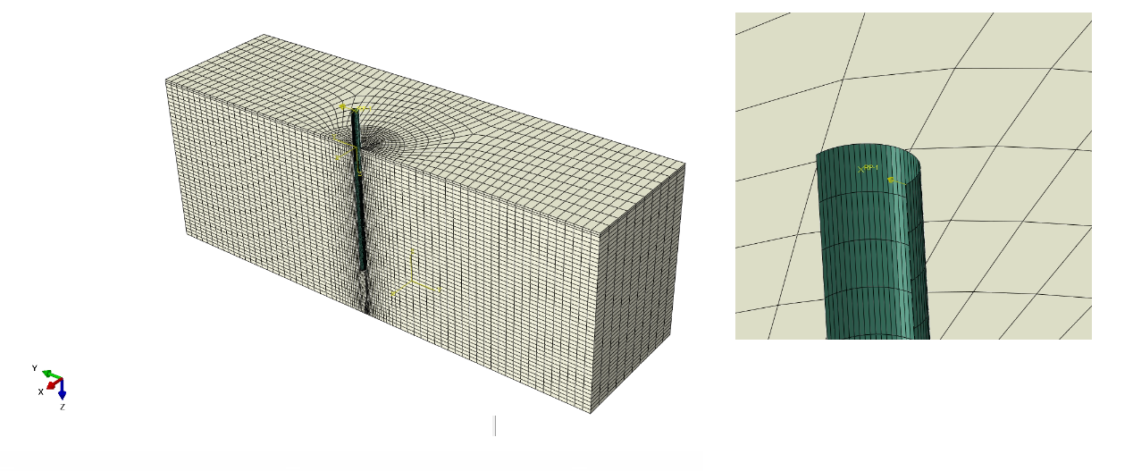
The parameter of the pile and the soil are same as mentioned  in the study of Hong et al. The soil is modelled as a solid entity with C3D8P element, and Pile is modelled as S4 shell element.

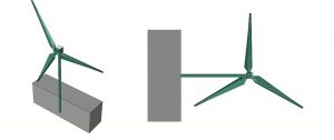
Geometry of the pile and soil used in model

1. First step in the modelling procedure is the definition of the material. The pile is modelled as semi rigid material with relative pile stiffness in between the rigid and flexible pipe. The relative soil pile stiffness depends on the flexure rigidity of the pile , soil elastic modulus and the imbedded depth of the pile. The flexure rigidity of the pile is calculated using elastic modulus of the pile and its moment of area. Similar the soil elastic modulus is calculated from the undrained shear strength which is taken as 400 time of its undrained shear strength at the middle height. Undrained shear strength is calculated as 10 Kpa as calculated by the study of Hong et al. The pile flexure rigidity  of 195 N·m2 is taken in the study. s we already know the moment of of the pile, from this we can calculate the the elastic modulus of pile which comes out to be around 52 MPA
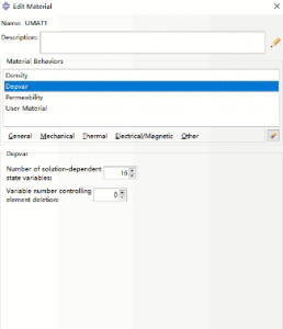
2. The second phase and the most critical phase of the modelling is defining the material of the soil. Soil is modelled using a user subroutine UMAT available at soilmodels.com .   The specific gravity of 16.5 kN/m is used in the model. In order to call the output variable from the subroutine, DEPVAR function is called in the material section in abaqus and its value is set to 16. The detail of these parameters are available at link .
3. 
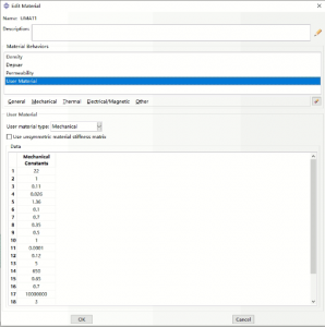
4. In the next phase material parameter of the hypoplastic soil are defined . The detail of these parameters are found at http://web.natur.cuni.cz/uhigug/masin/plaxumat/node6.html.

5. In the next phase the most important portion is definition of initial void ratio or OCR in the model. Regarding the selection of the OCR or void ratio the following statement is mentioned in the book Modelling of Soil Behaviour with Hypoplasticity by David Mašín[2] ”Both methods of void ratio initialization are applicable for clays, and they can be
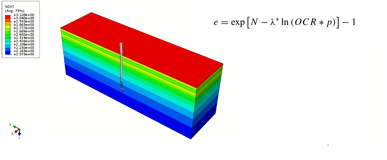
selected depending on their character. In general, OCR-based initialization is more suitable for softer clays. In stiff clays, it is often more relevant to specify a constant void ratio in the clay layer”. In our case as we are dealing with softer clay so we opted for OCR based initialization. In this regard different layers were defined in the soil and OCR was assigned to each layer individually by assigning the value to  PROPS[22] in the material section of the soil. The value of the OCR for the kaolin clay used in our study and its variation with the depth is taken from the Hongetal [3] as shown in figure. Remember initialization of the OCR must be done using SDVINI subroutine which is used in coordination with the  UMAT subroutine. The SDVINI  subroutine pattern is available  in the comment section of Hypoplasticity UMAT download blog. Remember as we are using OCR based initialization, instead of assigning values to SDV7 which is used as initial state variable to call OCR, PROPS[22] should directly be called in this subroutine.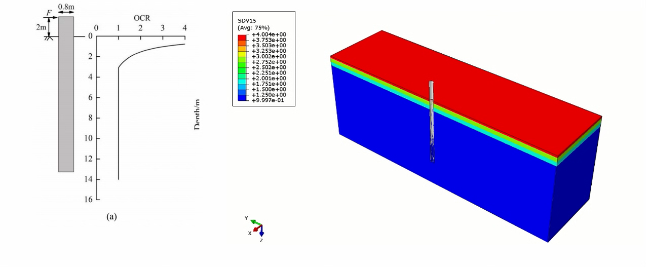 

6. As we are using OCR based initialization model will itself calculate the void ration based on the following equation. Remember OCR is called via SDV7 variable and its output is available at SDV15. and SDV7 output shows the calculated void ratio from the give value of OCR. The equation used in the model can be found at [2]  and its calculation is depicted below.

7. After initialization the first step is assigning the gravity load to the model based on the centrifuge scaling law. As in our case the model is scaled to 1:40 , so an initial acceleration of 40 g is applied as a geostatic stress via geostatic step. Following are the parameters that are effect by the scaling of the model.

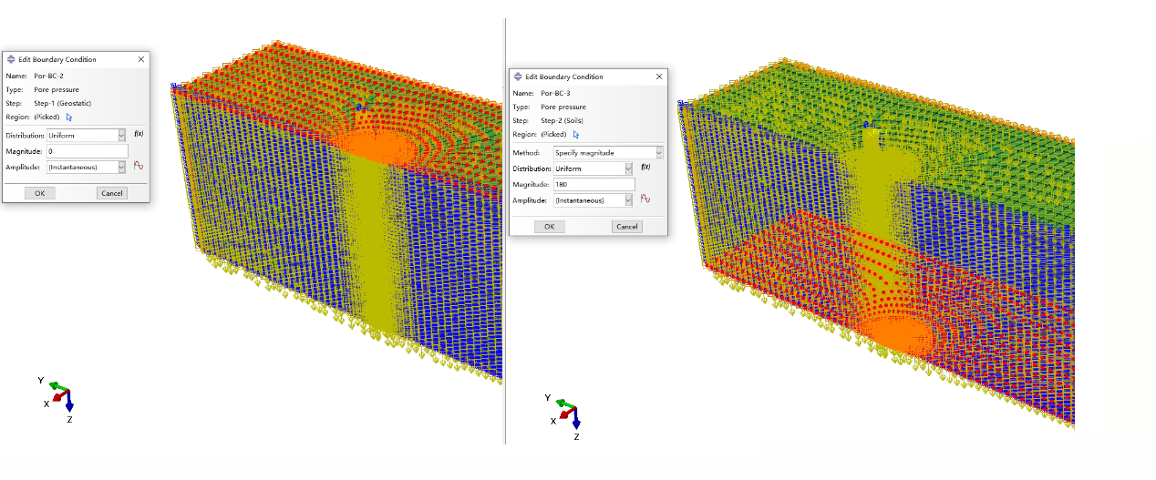
8. In the 2nd step a coupled consolidation analysis is performed, and a water table is maintained at the upper and lower face of the soil by specifying value 0 and 180 KPa respectively. This done via selecting  soil step and the consolidation time is selected according to the centrifuge scaling law.

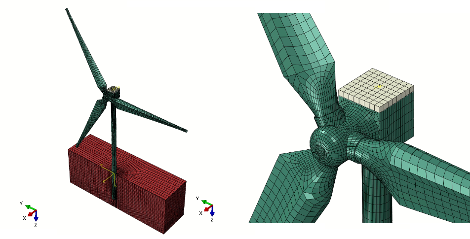
8. In the last step a lateral is applied to the one corner of the pile as shown in figure, a total of 100 constant load cycles are applied and the soil stiffness degradation pattern in observed . This model is helpful is assessing the response of the soil under earthquake or cyclic load.

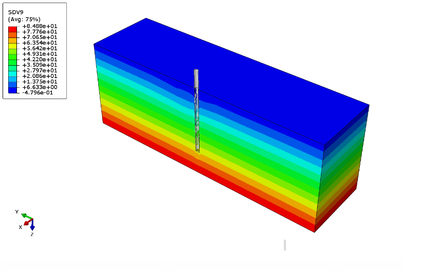
9. Below is the effective stress calculation performed by the model. Effective stress calculation is performed by taking average of deviatoric stresses specified using geostatic step in the model . SDV9 variable represent the deviatoric stress in the subroutine code UMAT

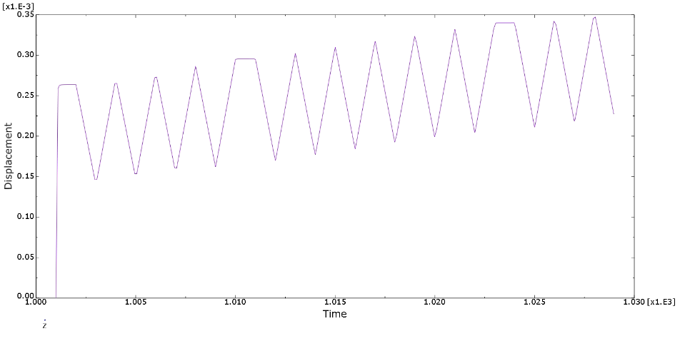
10.  Figure below depicts the pile head displacement under constant load cycle. Remember if you want to take stiffness anisotropy into account than you need to initialize the the vertical component of the strain tensor in the user subroutine  via SDVINI subroutine.

Good luck. Any question please do let me know in the comment box

Thank you very much

Arsalan

References

[1] Hypoplasticity for beginners by Wolfgang Fallin.

[2] Modelling of Soil Behaviour with Hypoplasticity by David Mašín.

[3] hong et al. Cyclic lateral response and failure mechanisms of semi-rigid pile in soft clay: centrifuge tests and numerical modelling.