The study aims to model the corrosion behaviors  of dental implant using Phase field paradigm. Film rupture, dissolution and repassivation model is used to predict the corrosion behavior. The Film Rupture, Repassivation, and Dissolution (FRDR) model is a theoretical framework that describes the corrosion process of a metal in a corrosive environment. It involves three stages:

1. Film Rupture: The protective oxide layer on the metal surface is damaged, allowing corrosive agents to penetrate.
2. Repassivation: The metal reacts with the environment to form a new protective oxide layer.
3. Dissolution: The metal dissolves into the surrounding environment. The FRDR model provides a useful way to understand and predict corrosion behavior, as it considers both the chemical and physical processes that occur during corrosion.

Each of this stage is modelled using UEL subroutine. For detail on the model Please do visit https://www.empaneda.com/codes/ to check the detail of this model. Here we will explain the modelling procedure using UEL subroutine in Abaqus and overview of UEL is presented. The code used here is slightly modified in order to transfer the stress tensor from UEL to UMAT. Here is step by step modelling procedure. The procedure used here is successfully tested for Plain strain, plain stress and Shell elements. When using user-defined elements in Abaqus, it is difficult to see information about what’s happening at each integration point. To solve this problem, a dummy mesh made of normal Abaqus elements can be created. This dummy mesh can be used to store information about what’s happening at each integration point, making it easier to understand and visualize the results of the simulation. To create the dummy, first of all .inp file of model is created and the assembly nodal point data is copied to excel file and create the same mesh with offset double of the original value. Here is screenshot

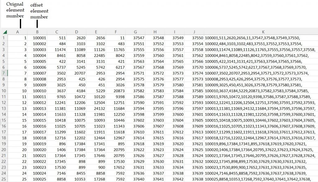
Now after creation of the offset element we need to incorporate this into the final mesh but before that we need to define the degree of freedom associated with the element in UEL and as well are dealing with two new parameters i.e. phase field and concentration.  So we need to assign them as degree of freedom but make sure these degree of freedom is not active in element. Here is the degree of freedom look like for different element. For Plain strain element , the lines look like

*User element, nodes=8, type=U1, properties=12, coordinates=2, var=96
1,2
1,3
1,11

In this the first line depicts the active degree of freedom in element. and phase field is applied using 3 degree of freedom and concentration is applied using 11, temperature degree of freedom. For shell element it would look like

*User element, nodes=8, type=U1, properties=12, coordinates=2, var=96
1,2,3,4,5,6
1,7
1,11

*User element, nodes=8, type=U1, properties=12, coordinates=2, var=96
1,2,3,4,5,6
1,7
1,11

For 3D element i.e. C3D8, the convention look like

*User element, nodes=8, type=U1, properties=12, coordinates=2, var=96
1,2,3
1,4
1,11

Now after degree of freedom we need to incorporate this into the model. This is done by adding the lines after the part module as shown in figure.

s

After the end of the assembly module we need to define the material properties. For material properties and calibration, Please refer to the article of https://doi.org/10.1016/j.jmps.2020.104254. The addition of the material section and the dummy mesh look like

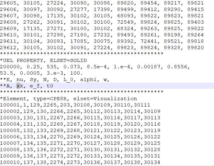
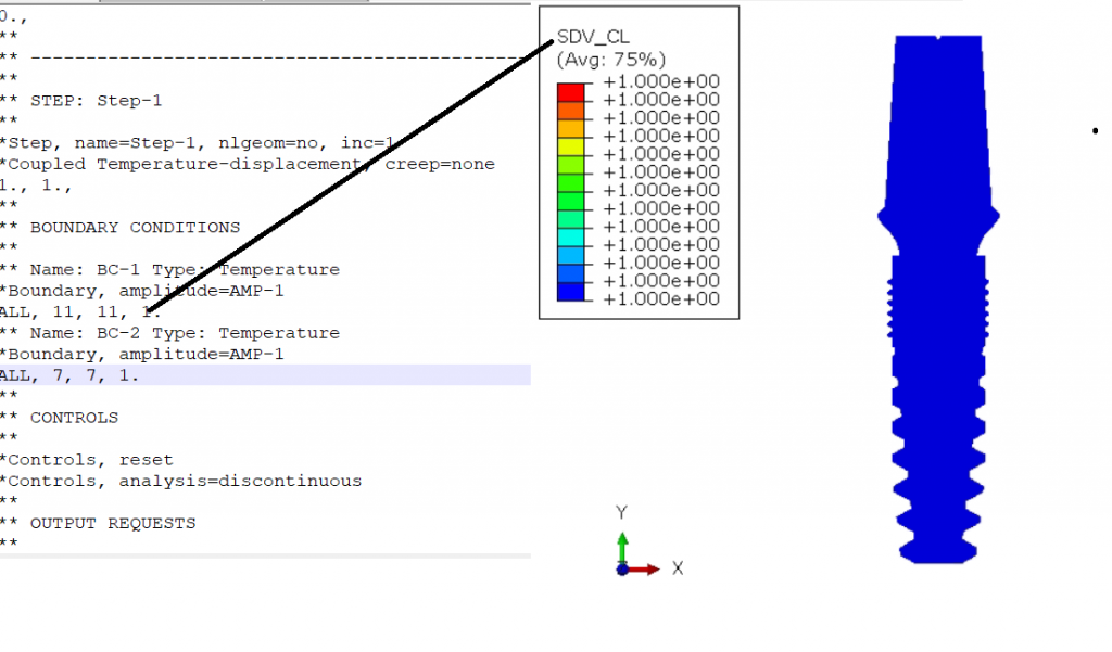
After the element definition is completed , we need to define the the steps in order to apply the FRDR modelling process. The first step is applying the concentration and phase field paradigm in the model. As the calibration of the phase field is one in away its value is 1 in metal and 0 in electrolyte. and at the interface the values ranges from 0-1. So this is done by  initializing the value of the phase field paradigm and concentration. Here is how the input file and the the results look like

After applying the concentration and phase field to the model, we will start with Film Rupture procedure. As we know that metals are covered with nano layered oxides layers so we need to apply the force is the form of displacement in order to rupture the interface oxide layer. That how the step definition and the stress pattern look like :

In the next phase we will apply the phase field and concentration with decreasing amplitude in order to model the dissolution of the fluid into the metal phase. This is how the step definition look like:

Results

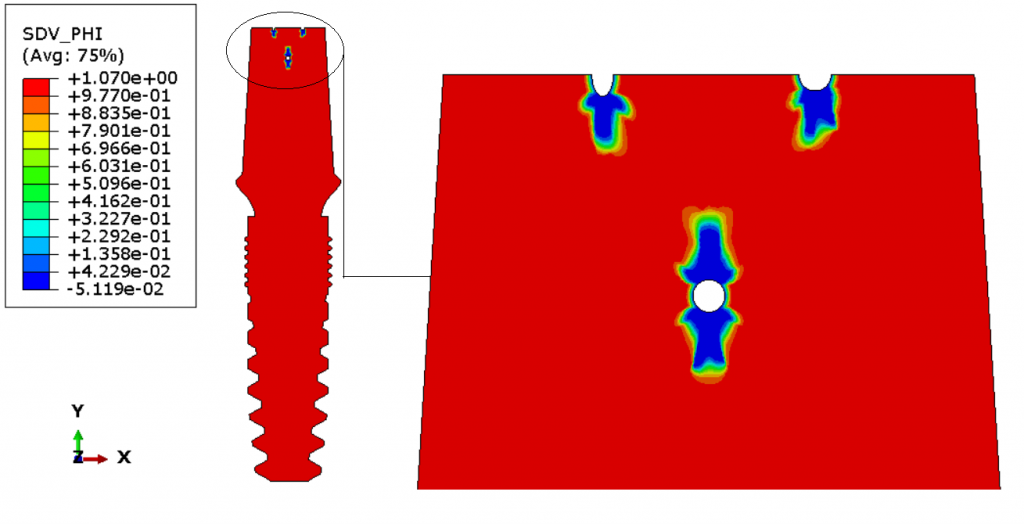
The procedure is carried out for single pit and multiple pit model. The pit to crack transition model is shown as under :

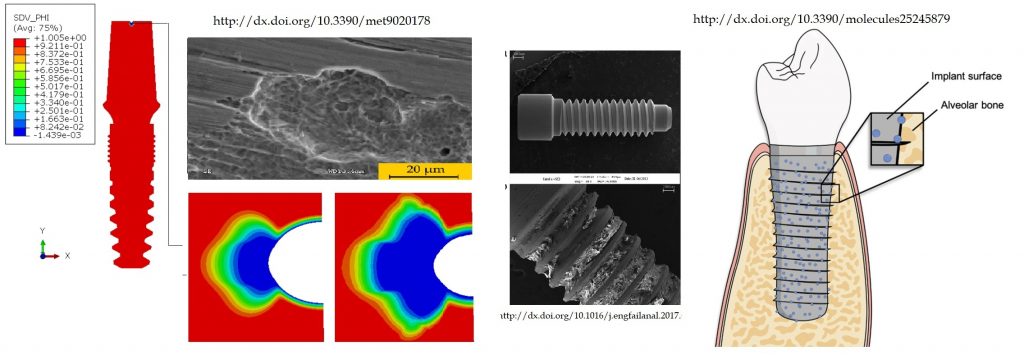
Similarly for the multiple pit model , the multiple pit model is tested against various pit shape , including simi-ellipsoidal, semi-circular, and circular shape. The pit to crack transition model look like :

Now a insight of UEL subroutine is presented alongside the extension of 2D UEL subroutine to be used for 3-Dimensional element. The constitutive equation of UEL look like:

K∆U (at certain time )=R-F corresponds to F=Kx. whereas, K is the stiffness matrix that need to be provided in the UEL and is termed as “amatrix” in UEL subroutine. ∆U is the output of the UEL and “F”” is the load vector provided by the UEL. To obtain the load vector the “F” the subroutine “”RHS”” is used. The basic step is writing the UEL subroutine are as under :

1. Define Shape Function: The shape function defines the relationship between the local and global coordinate systems. It is used to interpolate the unknown nodal values at the integration points.
2. Derivatives of Shape Function: The derivatives of the shape function are used to calculate the deformation of the element.
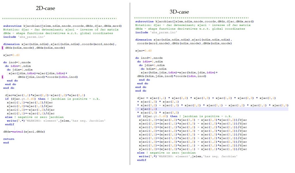
3. Jacobian Matrix: The Jacobian matrix is used to transform the local derivatives of the shape functions to the global derivatives.
4. Derivatives of Jacobian Matrix: The derivatives of the Jacobian matrix are used in the calculation of the B-matrix, which relates the nodal degrees of freedom to the element strains.
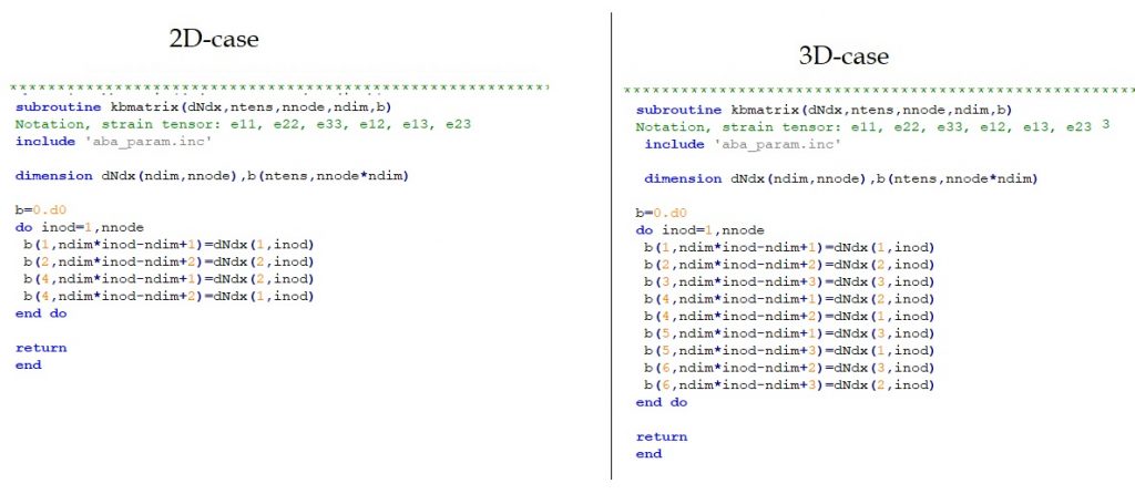
5. B-Matrix: The B-matrix is used in the calculation of the element stiffness matrix. It relates the nodal degrees of freedom to the element strains.
6. Stiffness Matrix: The stiffness matrix is used to calculate the internal forces in the element. It is calculated by multiplying the B-matrix by the element material properties and integrating over the element volume.
7. Internal Stress and Internal Force: Finally, the internal stress and internal force are calculated by multiplying the element strains and stresses, respectively, by the element volume. The results are then assembled into the global stiffness matrix and force vector.

So UEL subroutine starts from defining the interpolation function of element i.e. if we know a stress at corner in the element than how to calculate the stress at the middle of element. This is done by defining the shape function subroutine.  The shape function subroutine for 2D cases from the study and its possible extension to 3D may look like:

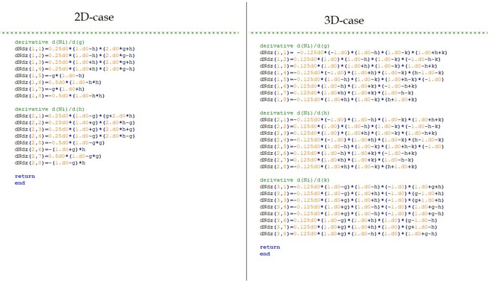
The derivate of the shape function and its possible extension to 3D may look like:

The Jacobian matrix for 2D-cases and 3D cases are shown as under:

The b-matrix and its extension from 2D to 3-dimensional case may possibly look like

 

Apart from this we have to change the dimension of the stress and strain tensor in the in the UEL subroutine. Also we need to change the degree of freedom ndoefl depends on element degree of freedom, ndim from2 to 3 and integration point numbering based on the element under consideration.

In the upcoming blog i will explain the effect of corrosion on the fatigue performance of biomedical implants.

 

Thank you very much everyone for reading my blog. If you have any question or suggestion or feedback, please reach me at:

Email# arsalanmuhammadahmad@yahoo.com’

Whatsaap# +92-315-977-9633